Lists are the basic ordered and mutable data collection type in Python. They can be defined with comma-separated values between square brackets; for example, here is a list of the first several prime numbers:

L = [2, 3, 5, 7]

Lists have a number of useful properties and methods available to them. Here we'll take a quick look at some of the more common and useful ones:

Length of a list

len(L)

4

Append a value to the end

L.append(11)
L

[2, 3, 5, 7, 11]

Addition concatenates lists

L + [13, 17, 19]

[2, 3, 5, 7, 11, 13, 17, 19]

sort() method sorts in-place

L = [2, 5, 1, 6, 3, 4]
L.sort()
L

[1, 2, 3, 4, 5, 6]

In addition, there are many more built-in list methods; they are well-covered in Python's online documentation.

While we've been demonstrating lists containing values of a single type, one of the powerful features of Python's compound objects is that they can contain objects of any type, or even a mix of types. For example:

L = [1, 'two', 3.14, [0, 3, 5]]

This flexibility is a consequence of Python's dynamic type system. Creating such a mixed sequence in a statically-typed language like C can be much more of a headache! We see that lists can even contain other lists as elements. Such type flexibility is an essential piece of what makes Python code relatively quick and easy to write.

So far we've been considering manipulations of lists as a whole; another essential piece is the accessing of individual elements. This is done in Python via indexing and slicing, which we'll explore next.

List indexing and slicing

Python provides access to elements in compound types through indexing for single elements, and slicing for multiple elements. As we'll see, both are indicated by a square-bracket syntax. Suppose we return to our list of the first several primes:

L = [2, 3, 5, 7, 11]

Python uses zero-based indexing, so we can access the first and second element in using the following syntax:

L[0]

2

L[1]

3

Elements at the end of the list can be accessed with negative numbers, starting from -1:

L[-1]

11

L[-2]

7

You can visualize this indexing scheme this way:

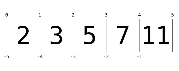
Here values in the list are represented by large numbers in the squares; list indices are represented by small numbers above and below. In this case, L[2] returns 5, because that is the next value at index 2.

Where indexing is a means of fetching a single value from the list, slicing is a means of accessing multiple values in sub-lists. It uses a colon to indicate the start point (inclusive) and end point (non-inclusive) of the sub-array. For example, to get the first three elements of the list, we can write:

L[0:3]
[2, 3, 5]

Notice where 0 and 3 lie in the preceding diagram, and how the slice takes just the values between the indices. If we leave out the first index, 0 is assumed, so we can equivalently write:

L[:3]
[2, 3, 5]

Similarly, if we leave out the last index, it defaults to the length of the list. Thus, the last three elements can be accessed as follows:

L[-3:]
[5, 7, 11]

Finally, it is possible to specify a third integer that represents the step size; for example, to select every second element of the list, we can write:

L[::2]  # equivalent to L[0:len(L):2]
[2, 5, 11]

A particularly useful version of this is to specify a negative step, which will reverse the array:

L[::-1]
[11, 7, 5, 3, 2]

Both indexing and slicing can be used to set elements as well as access them. The syntax is as you would expect:

L[0] = 100
print(L)

[100, 3, 5, 7, 11]

L[1:3] = [55, 56]
print(L)

[100, 55, 56, 7, 11]

A very similar slicing syntax is also used in many data science-oriented packages, including NumPy and Pandas.

That was a brief guide to Python lists. After getting a grasp on them, you can begin to learn about Python tuples.